CS224n Learning Notes--Word Vectors

Stanford CS224n Learning Notes 1: Word Vectors

This blog is just my learning notes of Stanford CS224n so I used many expressions and graphs from slides and lecture readings. If there are copyright problems, please contact me.

1. Introduction of Word Vectors

Finally started this course at the end of November. I will update this series of learning note as well as I finished learning a unit of CS224n course. Okay, let’s get started!

1.1. WordNet

At the very beginning, People use WordNet to represent the relationship of synonyms and hypernyms between words. However, there are some problems:

• This method will miss nuance.
  • According to the slides of this lecture, “proficient” is listed as a synonym for “good” but this is true only in some context.
• The WordNet won’t be updated as time move on.
• Very subjective
• Requires human labor
• Can’t compute accurate word similarity

1.2. One-hot Vector

So we should represent word with a new method. People use one-hot vectors to represent a word. The dimension of the vector is the size of vocabulary and each element represents a word.

• e.g.: computer = [0 0 0 0 0 1 0 0 0 0]; air = [1 0 0 0 0 0 0 0 0 0]
  • So the sixth position is computer and the first element is air

This still have some problems. We can’t know the relationship between one word and another since we just use one number to say if this “is the word” or not. So we should get someway learn to encode similarity in the vectors themselves.

1.3. Word Vectors

According to Distributional semantics: A word’s meaning is given by the word that frequently appear close-by. This means that if a word appears in a specific context, its synonyms will be likely to appear in the same context. So we can use context to find the similarity of words.

2. Method to Find Word Vectors

2.1. Co-occurrence Matrix

The first thing we can do is to count “what words are sitting around me”(imagine you are a word). We use a window that let us to see just a small number of words before and after the word of interest instead all the words before or after it.

Here’s an example from the reading of this course:

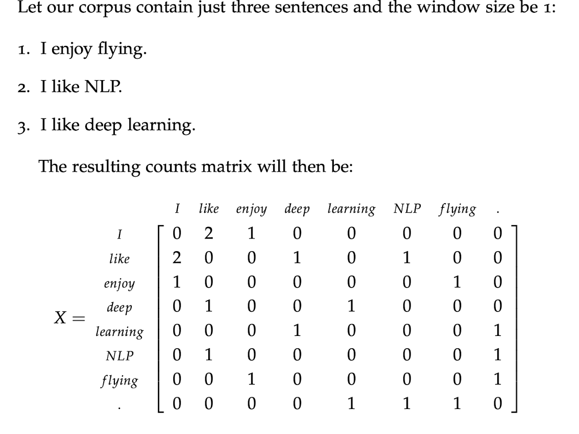
But this matrix is too sparse so we need to let it become denser. Here we use SVD to reduce the dimension. We use $U$ as word vector.

Code(From Assignment)

Constructing Co-occurrence Matrix

def compute_co_occurrence_matrix(corpus, window_size=4):
    """ Compute co-occurrence matrix for the given corpus and window_size (default of 4).
    
        Note: Each word in a document should be at the center of a window. Words near edges will have a smaller
              number of co-occurring words.
              
              For example, if we take the document "START All that glitters is not gold END" with window size of 4,
              "All" will co-occur with "START", "that", "glitters", "is", and "not".
    
        Params:
            corpus (list of list of strings): corpus of documents
            window_size (int): size of context window
        Return:
            M (numpy matrix of shape (number of corpus words, number of corpus words)): 
                Co-occurence matrix of word counts. 
                The ordering of the words in the rows/columns should be the same as the ordering of the words given by the distinct_words function.
            word2Ind (dict): dictionary that maps word to index (i.e. row/column number) for matrix M.
    """
    words, num_words = distinct_words(corpus)
    M = np.zeros((num_words, num_words))
    word2Ind = {}
    
    # ------------------
    # Write your implementation here.
    for i in range(0, len(words)):
        word2Ind[words[i]] = i
    for s in corpus:
        for i in range(0, len(s)):
            center_word = s[i]
            for j in range(i-window_size, i + window_size + 1):
                if j >= 0 and j != i and j < len(s):
                    M[word2Ind[center_word], word2Ind[s[j]]] += 1
            
    # ------------------

    return M, word2Ind

Perform SVD

def reduce_to_k_dim(M, k=2):
    """ Reduce a co-occurence count matrix of dimensionality (num_corpus_words, num_corpus_words)
        to a matrix of dimensionality (num_corpus_words, k) using the following SVD function from Scikit-Learn:
            - http://scikit-learn.org/stable/modules/generated/sklearn.decomposition.TruncatedSVD.html
    
        Params:
            M (numpy matrix of shape (number of corpus words, number of corpus words)): co-occurence matrix of word counts
            k (int): embedding size of each word after dimension reduction
        Return:
            M_reduced (numpy matrix of shape (number of corpus words, k)): matrix of k-dimensioal word embeddings.
                    In terms of the SVD from math class, this actually returns U * S
    """    
    n_iters = 10     # Use this parameter in your call to `TruncatedSVD`
    M_reduced = None
    print("Running Truncated SVD over %i words..." % (M.shape[0]))
    
        # ------------------
        # Write your implementation here.
    svd = TruncatedSVD(n_components=k, n_iter=n_iters, random_state=42)
    svd.fit(M)
    M_reduced = svd.components_
    
        # ------------------


    print("Done.")
    return M_reduced.T

Problems

• The dimensions of the matrix change very often(new words are added very frequently and corpus changes in size)
• The matrix is extremely sparse since most words do not co-occur
• The matrix is very high dimensional in general
• Quadratic cost to train(SVD)
• Requires the incorporation of some hacks on X to account for the drastic imbalance in word frequency

2.2. Word2Vec

Word2Vec can resolve many problems mentioned above. It comes from the training process of Language Model as a parameter.

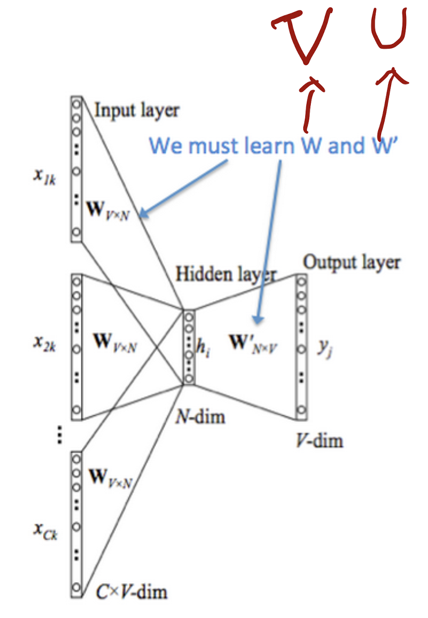
Continuous Bage of Words Model(CBOW)

• We use this algorithm to predict a center word from the surrounding context
• For each word, we use 2 vectors $u$(when the word is in the context) and $v$(when the word is in the center) to represent it.

Notation for CBOW Model:

• $X$: input(one-hot vector matrix)

• $w_i:$ Word $i$ from vocabulary $V$

• $\mathcal{V}\in R^{n \times|V|}$: Input word matrix

• $v_i$: i-th column of $\mathcal{V}$, the input vector representation of word $w_i$

• $\mathcal{U}\in R^{|V|\times n}$: Output word matrix

• $u_i$: i-th row of $\mathcal{U}$, the output vector representation of word $w_i$

Steps

1. We generate our one hot word vectors for the input context of size $m:(x^{c-m},…,x^{c-1},x^{c+1},…,x^{c+m})\in R^{|V|}$

2. We get our embedded word vectors for the context$(v_{c-m}=\mathcal{V}x^{c-m}, v_{c-m+1}=\mathcal{V}x^{c-m+1},…,v_{c+m}=\mathcal{V}x^{c+m}\in R^n)$

   • Since $x^i$is one hot vector, so this equation just selects $v_i$ from $\mathcal{V}$

3. Average these vectors to get $\hat{v}=\frac{v_{c-m}+…+v_{c+m}}{2m}\in R^n$

4. Generate a score vector $z=\mathcal{U}\hat{v}\in R^{|V|}$

   • This step actually computing the similarity between each word in $V$ and the given context $\hat{v}$

5. Turn the scores into probabilities $\hat{y}=softmax(z)\in R^{|V|}$

   • $\text{softmax}(\hat{y_i}) = \frac{e^{\hat{y_i}}}{\Sigma_{k=1}^{|V|}e^{\hat{y_k}}}$

6. We desire our probabilities generated, $\hat{y}\in R^{|V|}$, to match the true probabilities,$y\in R^{|V|}$, which also happens to be the one hot vector

Objective function

We use cross-entropy as our loss function since if $\hat{y}_{true}=1$, loss = 0, if $\hat{y}_{true}\approx0$, loss is very big.( $\hat{y}_{true}$ is the position where the correct word’s one hot vector is 1)

$$H(\hat{y},y)=-\Sigma^{|V|}_{j=1}y_jlog(\hat{y_j})=-y_ilog(\hat{y_i})\text{(since $y$ is one hot)}$$

So the objective is:

$$\begin{align} \text{minimize}J&=-logP(w_c|context)\\ &=-logP(u_c|\hat{v})\\ &=-log\frac{exp(u_c^T\hat{v})}{\Sigma_{j=1}^{|V|}exp(u_j^T\hat{v})}\\ &=-u_c^T\hat{v}+log\Sigma_{j=1}^{|V|}exp(u_j^T\hat{v})\\ \end{align}$$

Graph

Skip-Gram Model

Sikp-Gram Model is a method that use a single center word as the context to predict surrounding words. Its shares the idea of CBOW but just swap $x$ and $y$ of the model.

Steps

1. We generate our one hot input vector $x \in R^{|V|}$ of the center word
2. We get our embedded word vector for the center word $v_c=\mathcal{V}x \in R^n$
3. Generate a score vector $z=\mathcal{U}v_c$
4. Turn the score vector into probabilities, $\hat{y}=softmax(z)$. Note that $\hat{y}_{c-m},…,\hat{y}_{c-1}, \hat{y}_{c+1},…,\hat{y}_{c+m}$ are the probabilities of observing each context word
5. We desire our probability vector generated to match the true probabilities which is $y^{c-m},…,y^{c-1},y^{c+1},…,y^{c+m}$, the one hot vectors of the actual output.

Objective

$$\begin{aligned} \text { minimize } J &=-\log P\left(w_{c-m}, \ldots, w_{c-1}, w_{c+1}, \ldots, w_{c+m} | w_{c}\right) \\ &=-\log \prod_{j=0, j \neq m}^{2 m} P\left(w_{c-m+j} | w_{c}\right) \\ &=-\log \prod_{j=0, j \neq m}^{2 m} P\left(u_{c-m+j} | v_{c}\right) \\ &=-\log \prod_{j=0, j \neq m}^{2 m} \frac{\exp \left(u_{c-m+j}^{T} v_{c}\right)}{\Sigma_{k=1}^{|V|}exp \left(u_{k}^{T} v_{c}\right)} \ \\ &=-\sum_{j=0, j \neq m}^{2 m} u_{c-m+j}^{T} v_{c}+2 m \log \sum_{k=1}^{|V|} \exp \left(u_{k}^{T} v_{c}\right) \end{aligned}$$

Note

Only one probability vector $\hat{y}$ is computed. Skip-gram treats each context word equally: the models computes the probability for each word of appearing in the context independently of its distance to the center word.

• e.g.: [“I”, “like”, “NLP”]
  • In this case if we choose like as center word and window size of 1. We will predict $P(u_{like+1}|like)$ and $P(u_{like-1}|like)$ where $u_{like+1}$ means the word after like. Then we hope $P(u_{like+1}|like)$ is NLP‘s one hot vector and $P(u_{like-1}|like)$ is I‘s one hot vector.

Graph

2.3. Speed Up Training

As we can see, the objective function of these two methods, there are both an add term through all the vocabulary list, which is really computational expensive. So we need so way to approximate it.

Negative Sampling

Mikolov et al gave a method of Negative Sampling. The idea of this method us to sample from a noise distribution$(P_n(w))$ whose probabilities match the ordering of the frequency of the vocabulary. And to train a model that can specify if the pair of data is come from training data. That mean if two words come from the training data so the are more likely have relationships while if not, they may not correlated.

We use $P(D=1|w,c)$ as the probability that $(w,c)$ came from the corpus data and $P(D=0|w,c)$ will be the probability that $(w,c)$ did not come from the corpus data.

$$P(D=1|w,c,\theta)=\sigma(v_c^Tv_w)=\frac{1}{1+e^{(-v_c^Tv_w)}}\\ P=(D=0|w,c,\theta) = 1 - P(D=1|w,c,\theta)$$

So we can bulid a objective function that tries to maximize the probability of a word and context being in the corpus data if it indeed is, and maximize the probability of a word and context not being in the corpus data if they really did not. So $\theta$ is:

$$\begin{aligned} \theta &=\underset{\theta}{\operatorname{argmax}} \prod_{(w, c) \in D} P(D=1 | w, c, \theta) \prod_{(w, c) \in \tilde{D}} P(D=0 | w, c, \theta) \\ &=\underset{\theta}{\operatorname{argmax}} \prod_{(w, c) \in D} P(D=1 | w, c, \theta) \prod_{(w, c) \in \tilde{D}}(1-P(D=1 | w, c, \theta)) \\ &=\underset{\theta}{\operatorname{argmax}} \sum_{(w, c) \in D} \log P(D=1 | w, c, \theta)+\sum_{(w, c) \in \tilde{D}} \log (1-P(D=1 | w, c, \theta)) \\ &=\underset{\theta}{\operatorname{argmax}} \sum_{(w, c) \in D} \log \frac{1}{1+\exp \left(-u_{w}^{T} v_{c}\right)}+\sum_{(w, c) \in \bar{D}} \log \left(1-\frac{1}{1+\exp \left(u_{w}^{T} v_{c}\right)}\right) \\ &=\underset{\theta}{\operatorname{argmax}} \sum_{(w, c) \in D} \log \frac{1}{1+\exp \left(-u_{w}^{T} v_{c}\right)}+\sum_{(w, c) \in \tilde{D}} \log \left(\frac{1}{1+\exp \left(u_{w}^{T} v_{c}\right)}\right) \end{aligned}$$

Where $\tilde{D}$ is a false or negative corpus generated by randomly sampling.

Objective function

$$J=-\sum_{(w, c) \in D} \log \frac{1}{1+\exp \left(-u_{w}^{T} v_{c}\right)}-\sum_{(w, c) \in \tilde{D}} \log \left(\frac{1}{1+\exp \left(u_{w}^{T} v_{c}\right)}\right)$$

For skip-gram, our new objective function for observing the context word $c-m+j$ give the center word $c$ would be

$$-\log \sigma\left(u_{c-m+j}^{T} \cdot v_{c}\right)-\sum_{k=1}^{K} \log \sigma\left(-\tilde{u}_{k}^{T} \cdot v_{c}\right)$$

For CBOW, the objective is:

$$-\log \sigma\left(u_{c}^{T} \cdot \hat{v}\right)-\sum_{k=1}^{K} \log \sigma\left(-\tilde{u}_{k}^{T} \cdot \hat{v}\right)$$

where $\hat{v}=\frac{v_{c-m}+v_{c-m+1}+\ldots+v_{c+m}}{2 m}$

From above we can see that the add term reduce from $|V|$ to $K$.

Noise Distribution

The Noise Distribution is the Unigram Model raised to the power of 3/4. So that the less frequent word can have greater chance to be selected.

Hierarchical Softmax

Mikolov et al. also gave hierarchical softmax as a much more efficient alternative to the normal softmax. In parctice, hierarchical softmax tends to be better for infrequent words, while negative sampling work better for frequent words and lower dimensional vectors.

This method represent all words in the vocabulary. Each leaf of the tree is a word, and there is a unique path from root to leaf. In this model, each node in the path from root to leaf(no include the leaf) is a vector to be learned.

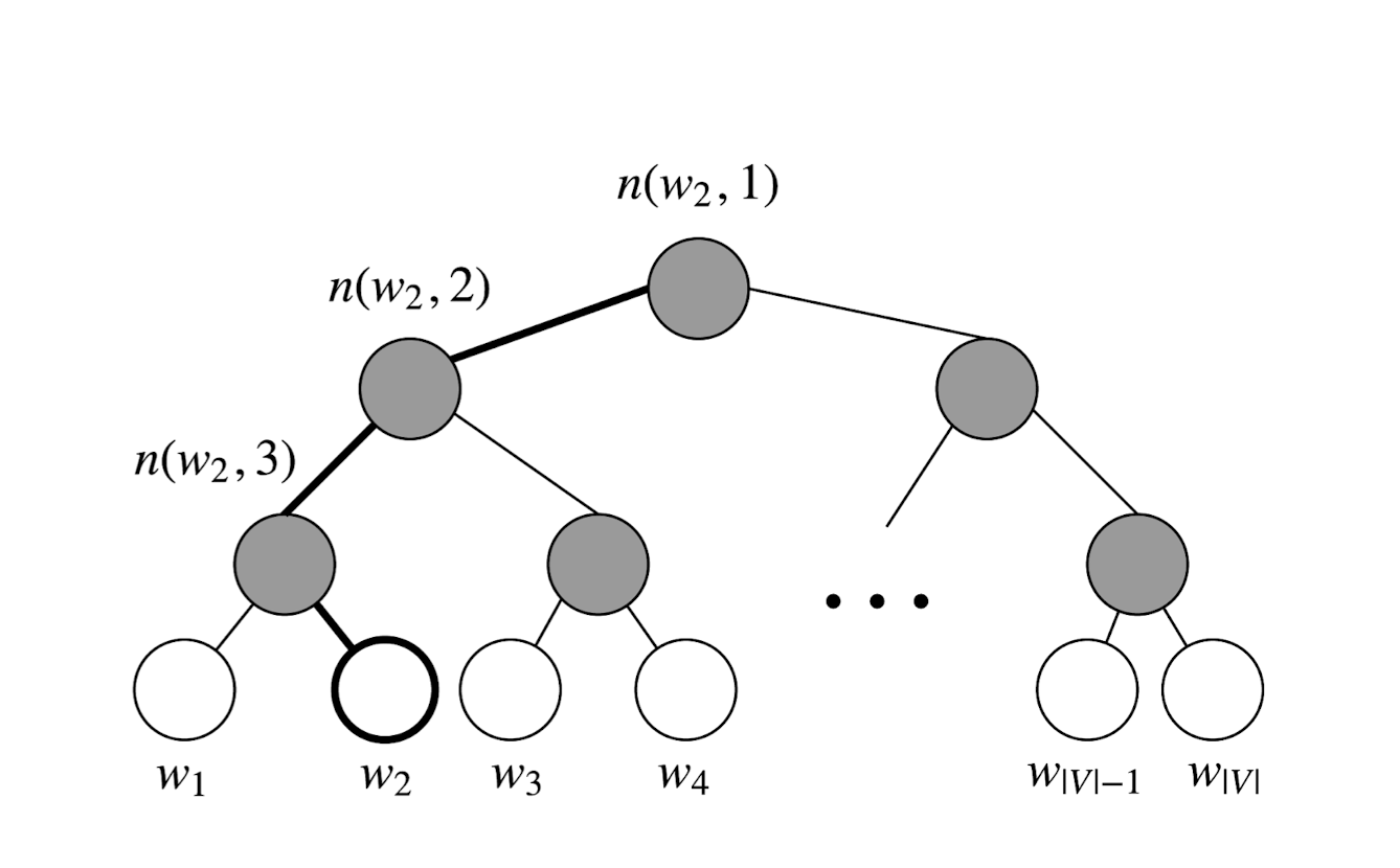
Notation

• $L(w)$: the number of nodes in the path from the root to the leaf $w$.
• $n(w,i)$: the i-th node on this path with associated vector $v_{n(w,1)}$.
• $ch(n(w,j))$: the left child of $n(w,j)$

We can compute the probability as:

$$P(w|w_i)=\Pi_{j=1}^{L(w)-1}\sigma([n(w,j+1)=ch(n(w,j))]·v^T_{n(w,j)}v_{w_i} )$$

where:

$$[x]=\left\{\begin{array}{l}{1 \text { if } x \text { is true }} \\ {-1 \text { otherwise }}\end{array}\right.$$

Then we can minimize the negative log likelihood $-logP(w|w_i)$.

This can turn O(|V|) to O(log|V|).

References

• $CS224n: Natural \ Language \ Processing\ with\ Deep\ Learning \ Lecture\ Notes:\ Part I \ \\Word Vectors I: Introduction, SVD\ and\ Word2Vec\ Winter \ 2019$