Data Science for Research Psychology Lecture Notes Part 1

Introduction

This is my lecture notes for UC Berkeley course Data Science for Research Psychology instructed by Professor Charles Frye. This post contains some basic data science and statistic knowledge. Most of the content showed following is from this course’s lecture slides with some of my understanding. You can check the original slides at here. If there are any copyright issues please contact me: haroldliuj@gmail.com.

There are some Chinese in this post, since I think my native language can explain those point more accurately. If you can understand Chinese, that’s great. If you can’t, those content won’t inhibit you from learning the whole picture. Feel free to translate it with Google!

Have a nice trip!

Lecture 02 Probability and Statistics

1. Probability

A measure quantifying the likelihood that events will occur

2. Probability Distributions

1. Discrete Distributions

Discrete distributions don’t need to have a finite number of observable values

2. Continuous Distributions

Density function

3. Statistics

1. Purposes

Descriptions or summarizations
- When we have the entire population of interest, all statistics is descriptive
Inference or moving beyond

2. Frequently used statistics

Mean
Median
Variance
Standard Deviation
Skew (-:right, +:left)

4. Law of Large Numbers

The valuse of descriptive statistic on a random sample gets closer to the value of that descripitive statistic
在多次重复实验的情况下事件的概率越等与其出现的频率

5. Bootstrapping

Since the statistics are varied after each sampling operation. We need some ways to measure the uncertainty of the statistics. The most easy way to do this is get more data and qunatify the uncertainty using intervals.

1. Confidence Interval

A confidence interval is any interval-valued statistic that has the property that for some known fraction of possible samples(这个区间有x%的概率包含总体的统计量)
when the 95% confidence interval is [0, 1], we are 95% sure that the value of the statistic on the true distribution is inside that interval.

2. Steps

def bootstrap_stat(s, stat_fun, n_boots):
    list = []
    for i in range(0, n_boots): #统计量的样本数
        sample = s.sample(frac=1, replace=True) #从已知的数据中重新抽样
        list.append(stat_fun(sample))#计算统计量 然后添加到list
    return list #此list用于以后数据分析(e.g. confidence Interval)

3. Understanding Bootstrapping

Bootstrapping是判断统计量的可信度的一种方法，因为统计量是从抽样得到的，会随着每一次抽样的不同而不同，但是根据大数定律，在获得足够多的统计量的样本后就能找到其真实的值，所以Bootstrapping 就是一种借用已有的数据通过重新抽样的方式来获取大量的统计量

Lecture 03 Models and Random Variables

1. Models

Unlike bootstrapping, models will genearte samples that don’t look ecxactly like data we observed

2. Frequently used distributions

1. Discrete

Binomial (二项分布)
- $f(x|n, p) = C_n^xp^x(1-p)^{n-x}$
Bernoulli(两点分布)
- $f(x|p)=p^x(1-p)^{1-x}$
- 二项分布是两点分布多次实验后的结果
Possion
- $f(x|\mu)=\frac{e^{-\mu}\mu^x}{x!}$
- Often used to model the number of events occurring in a fixed period of time when the times at which events occur are independent.
- 当二项分布n很大p很小时，近似服从泊松分布
- 泊松分布适合于描述单位时间（或空间）内随机事件发生的次数。如某一服务设施在一定时间内到达的人数，电话交换机接到呼叫的次数，汽车站台的候客人数，机器出现的故障数，自然灾害发生的次数，一块产品上的缺陷数，显微镜下单位分区内的细菌分布数等等。
DiscreteUniform(均匀分布)
- $f(x|lower, upper)=\frac{1}{upper-lower+1}$
Categorical(分布列) 参数 p概率和要为1
- $f(x|p) = p_x$

2. Continuous

Uniform
Flat/HalfFlat (Weakest prior)
Cauchy/HalfCauchy(Medium prior)
Normal
Exponential
- 描述泊松过程中事件之间的时间的概率分布
- 无记忆性：接下来公交来的概率和你等了多久并没有关系 $P(T>t+s|T>t)=P(T>s)$

Lecture 04 Parameters, Priors and Posteriors

1. Parameters

Different variable have different numbers and names of parameters but they all have them
Those parameters change the particular shape of the distribution of that random variable, while still keeping it within the same family

2. Marginal Distributions

假设有一个联合分布$P(x, y)$，其关于其中一个变量的边缘分布为 $P(X)=\Sigma_{y}P(x,y)=\Sigma_yP(x|y)P(y)$
The shapes of marginal distributions are not always given by the name of the variable
- e.g. If the variable X is a Foo, P(X) is not always going to be a member of the family Foo

3. Joint Distribution

$P(X, Y) = P(X|Y)P(Y)$

4. Conditional Distributions

5.`observed` Parameter

If we give a value to observed parameter, then calling pm.sample will draw from the conditional distribution $P(Signal|Measurement=observed\ data)$ instead of the marginal distribution $P(Signal)$
Put another way: the original model specified our uncertainty about the values of the signal and the measurement, and samples from it were used to numerically and visually represent that uncertainty.(Prior) Once we’ve observed the value of one of the random variables, the state of our knowledge changes, and so we’d like the samples to change to reflect that.(Posterior)

6. Implementation with PyMC

1. Steps

You write down a forwards model that

describes uncertainty about unknown quantities like parameters. This is the prior.

and then
explains what the distribution of the data _would be_, if you did know those unknown quantities. This is the likelihood.

pyMC can then “work backwards” and tell you
what your new beliefs
about the unknown quantities are,
once you’ve seen that data. This is the posterior.

These new beliefs are expressed as samples, drawn by pm.sample.

2. Bayes’ Rule

$\color{green}{p(\beta\lvert X)} = \color{goldenrod}{p(X\lvert\beta)} * \color{darkblue}{p(\beta)}\ /\ p(X)$

3. Sampling Functions

with pm.Model() as model:
    # random variable to model uncertainty about the truth before seeing data: the _prior_
    parameter_var = pm.SomeRandomVariable("prior_variable", parameter=value)  
    # random variable to model uncertainty in data, given parameters: the _likelihood_
    observed_var = pm.OtherRandomVariable("data_variable", paramter=parameter_var, observed=data_we_saw)
    
# samples to estimate uncertainty before seeing data
pripred_samples = pm.sample_prior_predictive(model=model)

with model:
    # samples to estimate uncertainty about the parameters after seeing data: the _posterior_
    post_samples_trace = pm.sample()

# samples to estimate uncertainty in what future data we might see:
postpred_samples = pm.sample_posterior_predictive(post_samples_trace, model=model)

pm.sample_prior_predictive(model)
- Samples to estimate uncertainty before seeing data
pm.sample()
- Samples to estimate uncertainty about the parameters after seeing data
pm.sample_posterior_predictive()
- samples to estimate uncertainty in what future data we might see

PS: Bootstrapping do not have priors

Drawbacks
- For some problems, there is no statistic of the data that supports the inference
- If we just look at likelihoods, we can end up making very silly inferences

4. Choosing Priors

1. Common Priors, and what they imply about your beliefs

Categorical: These are my beliefs about each possible value
(Discrete)Uniform: The value is between these two numbers
Normal: I know the value approximately, up to some spread
LogNormal: I know the order of magnitude approximately, up to some spread
Cauchy: I know almost nothing about this variable

2. Improper Priors

Flat: I know nothing about this variable, except it is a number (improper!)
HalfFlat: I know nothing about this variable, except that it’s positive (improper!)

5. Choosing Likelihoods

1. Common Likelihoods, and how they relate the parameters to data

Normal: values get more unlikely as they get further from mu, at a rate determined by 1/sd (aka tau)
Binomial: data is the outcome of a number of N independent attempts, each with probability p of occurring
Poisson: data is the outcome of independent attempts where N is large or infinite and p is small or infinitesimal, with mu=N * p.
Exponential: values get more unlikely as they get larger, at a rate determined by lam OR data is the time in between events in a memoryless process, occuring about lam every unit time
Laplace: values get more unlikely as they get further from mu in absolute difference, at a rate determined by 1/b

Note that some are mechanistic, others are not: the Normal is not particularly mechanistic, but the Poisson and Binomial are.

The Exponential might be mechanistic in some models, but not in others.

Lecture 05 Null Hypothesis Significance Testing

1. Null Hypothesis Significance Testing

1. Steps

Collect data
Come up with a model of “nothing interesting is happening in my data”(比如这两组数据均值没有区别)
- The model can be 1. resampling-based; 2 mathematical; 3. pyMC
- This is called the null model
Obtain the sampling distribution of the statistic from the model
Compare the value of the statistic observed on the data to the sampling distribution. If the observed value is “too extreme”, the test is positive and the result is “statistically significant” （计算比观察值更极端的情况的概率如果低于threshold 则判断为拒绝原假设）

2. Null Hypothesis Testing Cannot be Done with Basic Bootstrapping

Bootstrapping 是真实数据的模拟，而NHT是在Null成立的情况下检验是不是可以拒绝原假设，即便观察的数据否定原假设，我们还是需要通过模型来生成原假设为真时候的数据，而在原假设为假的情况下 bootstrapping 无法生存原假设为真的数据，所以Bootstrapping 不适合做假设检验

3. When the Value $p$ is Below a Threshold, we Reject the Null

4. $p$-value

$p$ is not the posterior probability of the Null
- We did not set a prior of $p$
$1-p$ is not the probability another run of same experiment would report the same finding
$p$ is the conditional probability of such an extreme statistic given that the Null is True

	F(原假设(e.g.无罪)为假)	T(原假设为真)
+(拒绝原假设)	True Positive Rate, Power, Sensitivity（判断有罪的人有罪）	False Positive Rate(把无辜的人当有罪), α
-(接受原假设)	False Negative Rate(放走有罪的人), β	True Negative Rate, Specificity

“P 值就是当原假设为真时，比所得到的样本观察结果更极端的结果出现的概率”。如果 P 值很小，就表明，在原假设为真的情况下出现的那个分布里面，只有很小的部分，比出现的这个事件（比如，Q）更为极端。没多少事件比 Q 更极端，那就很有把握说原假设不对了

2. Steps of Generic hypothesis testing(Not Null Hypothesis testing)(LJ)

Define a statistic of the observed data and calcualte thet chance of observing that statistic
Determine the chance your results would occur under that hypothsis
If the chance that your results or others like them would occur is sufficiently low, the hypothesis is rejected as falsified
最后算出概率后可以反推回观测值，比如投硬币案例中投xx次有xxxx次正面就可以证明硬币不均匀

3. t-Tests(关注两个组别是否存在差异)

1. Defining $t$

$t=\frac{\mu_a - \mu_b}{\sigma\sqrt{2/N_g}}$
where 𝜇𝐴 for a pandas series A is A.mean(), and 𝑁𝑔 is len(A), which is presumed equal to len(B). The other value the denominator, 𝜎, is the estimate of the group standard deviation and is given by:
$\sigma^2 = \frac{\sigma^2_A + \sigma^2_B}{2}$(Pooled standard deviation)
Degrees of freedom is the only parameter for the null distribution of $t$. In general, degrees of freedom is equal to the numer of datapoints from the dataset

4. Randomization Tests

1. Idea

The idea of a randomization test is to apply such a procedure to your data and see whether your data behaves more like two salt shakers or more like a salt and a pepper shaker.
We strip the labels off of the data, we put all of it into a bag, and then shuffle it around. Then, we pull it back out, sticking the labels back on randomly as we go.
适用于总体分布位置的小样本资料以及某些难以用常规方法分析资料的假设检验问题。主体思想是在小数据量情况下，如果两组样本分布相同，把他们混在一起重新抽样分布也还是相同，但是如果分布不同则混合后结果不会相同，在样本分布不同的时候通过这种混合抽样的方法算出来的统计量分布会与观察值产生比较大的偏差，从而证明两组样本分布不同

Lecture 06 Bayesian Inference

0. Bayes’ Rule

$p(\text{hypothesis}\vert \text{data}) = \frac{p(\text{data}\vert \text{hypothesis}) p(\text{hypothesis})}{p(\text{data})}$

1. Traditional Way

2. pyMC models

3. Iteratively Applying Bayes’ Rule

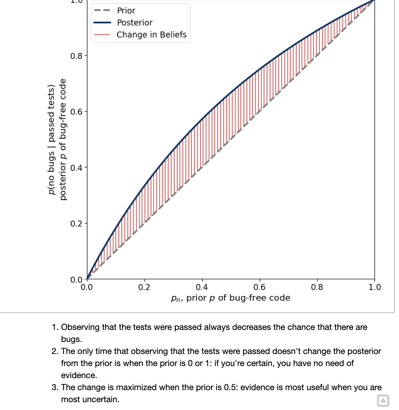
After the first tests have been passed is also before the second tests have been passed.
Therefore the posterior for the first set of tests is the prior for the second set of tests.

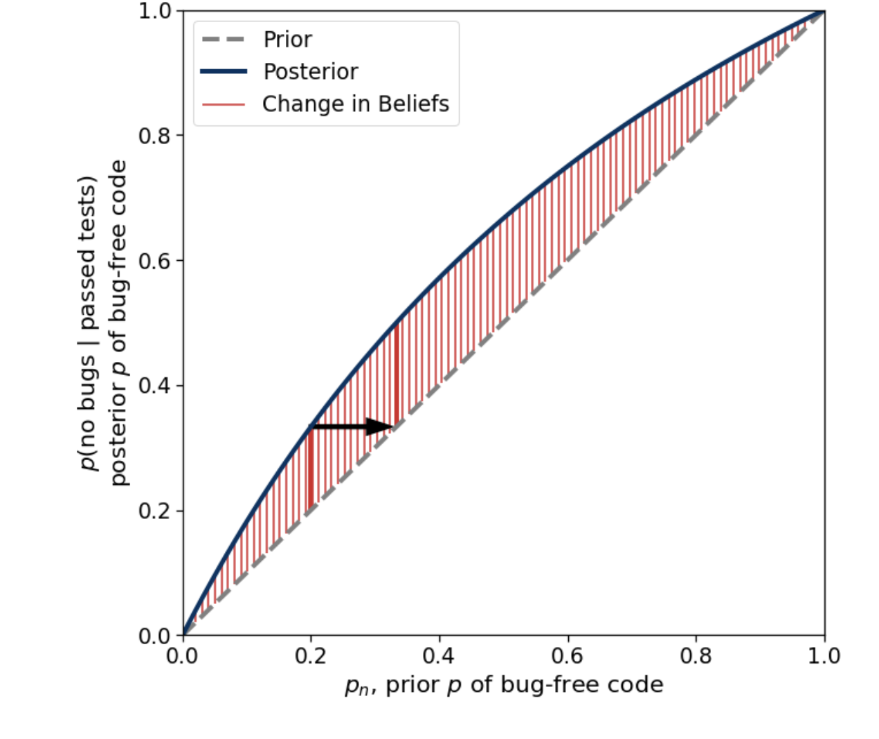
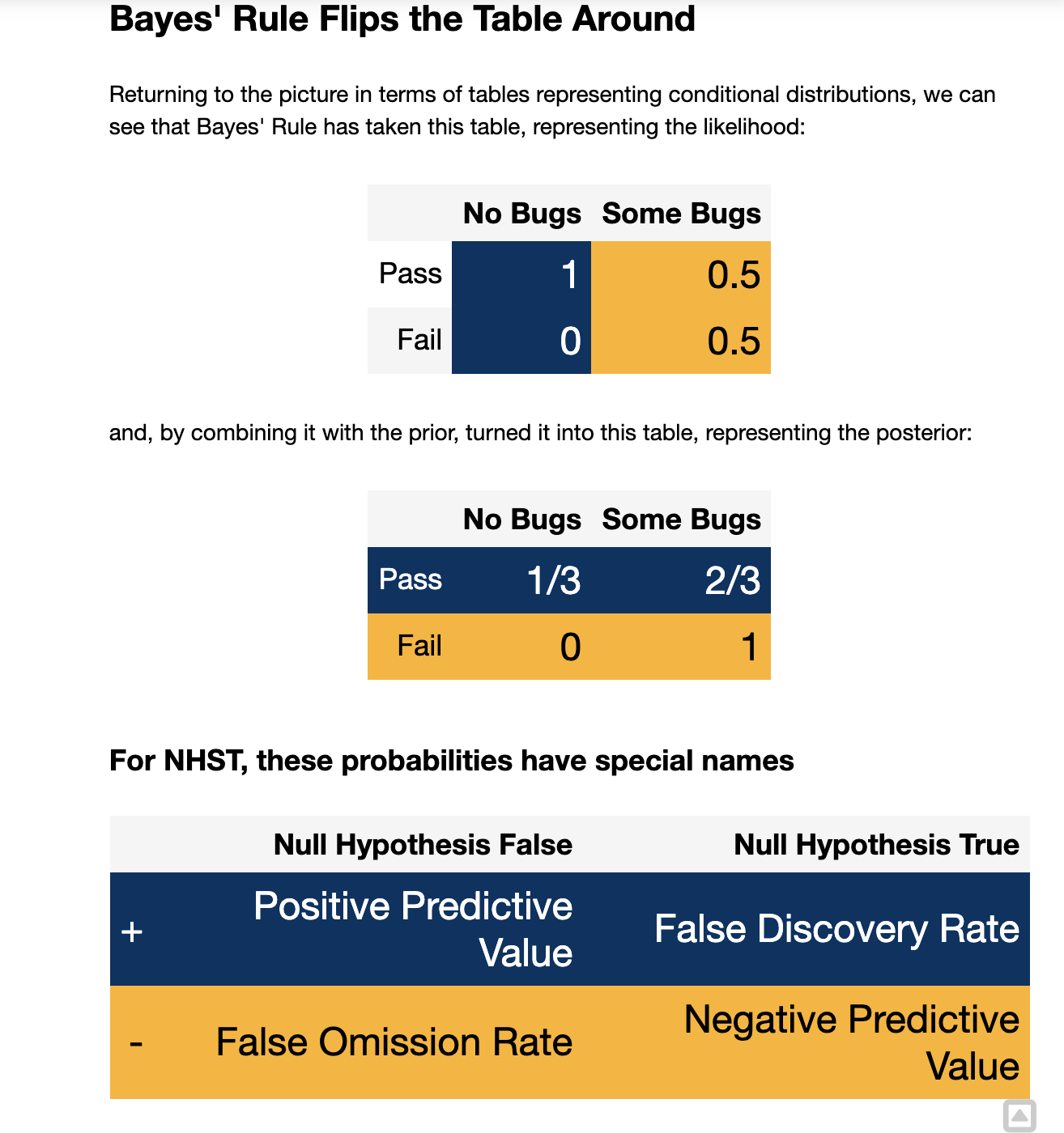
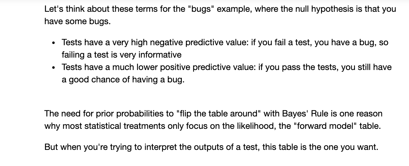
4. Bayes’ Rule Flips the Table Around

5. Credible Intervals

1. Definition

A Bayesian Credible Interval is any interval that covers some given percentage of the posterior density
- e.g. 95% Credible Interval covers 95% of the posterior. That is, if the 95% Credible Interval is (-1, 1) we believe there is 95% chance that the value lies between -1 and 1

2. Highest Posterior Density Intervals

The HPDI is the shortest credible interval

6. Point estimate

1. Ways to give estimate in Bayesian: By distribution

State the probability that it is true under my posterior.
Highest posterior density interval

Ps: It’s very unnatural to give point estimate in Bayesian inference

2. If have no choice, use MAP value

The closest thing to a Bayesian approach to providing point estimates is the maximum a posterior
MAP is the setting of all of the unkniwn variables that has the highest probability under the posterior
- That is, choose params to make
as high as possible
find_MAP

1 2	with sentiment_switch_model: sentiment_MAP = arrays_to_scalars(pm.find_MAP(start=sentiment_trace[-1]))

Introduction

Lecture 02 Probability and Statistics

1. Probability

2. Probability Distributions

1. Discrete Distributions

2. Continuous Distributions

3. Statistics

1. Purposes

2. Frequently used statistics

4. Law of Large Numbers

5. Bootstrapping

1. Confidence Interval

2. Steps

3. Understanding Bootstrapping

Lecture 03 Models and Random Variables

1. Models

2. Frequently used distributions

1. Discrete

2. Continuous

Lecture 04 Parameters, Priors and Posteriors

1. Parameters

2. Marginal Distributions

3. Joint Distribution

4. Conditional Distributions

5.observed Parameter

6. Implementation with PyMC

1. Steps

2. Bayes’ Rule

3. Sampling Functions

4. Choosing Priors

5. Choosing Likelihoods

Lecture 05 Null Hypothesis Significance Testing

1. Null Hypothesis Significance Testing

1. Steps

2. Null Hypothesis Testing Cannot be Done with Basic Bootstrapping

3. When the Value $p$ is Below a Threshold, we Reject the Null

4. $p$-value

2. Steps of Generic hypothesis testing(Not Null Hypothesis testing)(LJ)

3. t-Tests(关注两个组别是否存在差异)

1. Defining $t$

4. Randomization Tests

1. Idea

Lecture 06 Bayesian Inference

0. Bayes’ Rule

1. Traditional Way

2. pyMC models

3. Iteratively Applying Bayes’ Rule

4. Bayes’ Rule Flips the Table Around

5. Credible Intervals

1. Definition

2. Highest Posterior Density Intervals

6. Point estimate

1. Ways to give estimate in Bayesian: By distribution

2. If have no choice, use MAP value

5.`observed` Parameter